Factorial Design of Experiments: A practical case study. Part 2
Continuation from Part 1…
Last time, we talked a little bit about Design of Experiments (DoE), what it is, its main advantages and how it can help us for faster and improvement analysis of phenomena as well as gathering information to make the best possible decisions.
Moreover, we set a situation and prepared a factorial 23 DoE. Today, we are going to review the results and concluding about them.
As you remember, we had a machine that produces slugs and we needed to assure slugs meet specification of target weight ± 5%.
We defined three factors to study and our final DoE was set as follows. Our response variable is CP, so, in the following table you will already find results obtained after running the trials.
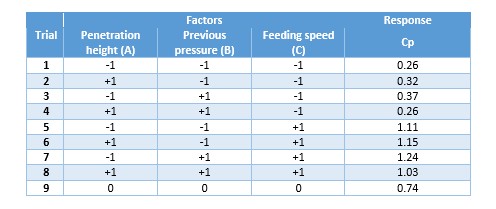
Now, let´s analyze results. For this exercise, we will use Minitab software.
Remember that we need to find out the optimum adjustment in the machine for getting slugs that meet specification of target weight ± 5%. So, let’s start!
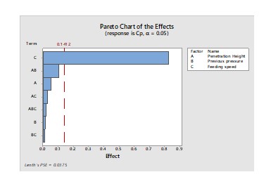
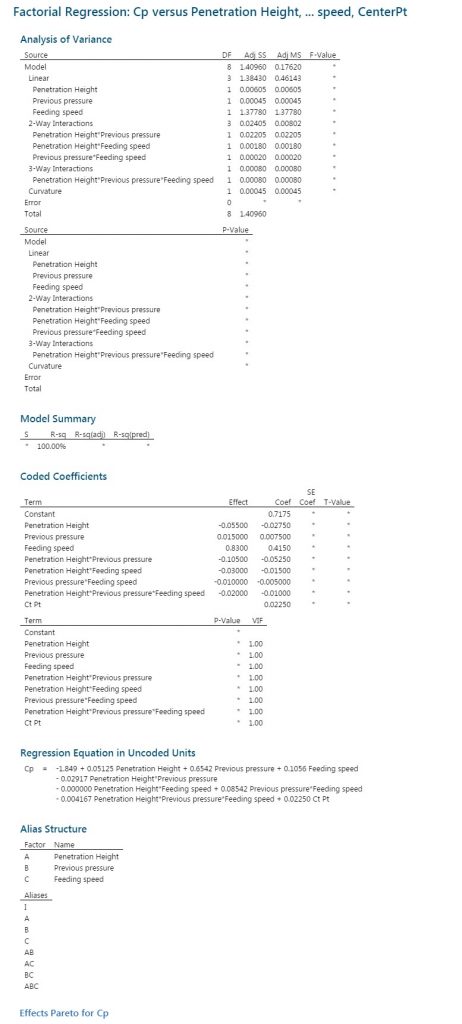
First than all, we need to evaluate which of the three factors are most important (or significant, statistically speaking) for getting the highest possible CP (ideally, ≥ 1.33). so, with the results we run an ANOVA. Minitab gives us the following data as well as a Pareto chart, which visually shows significant factors.
Other way to visualize which the main effects are is using a main effects plot:
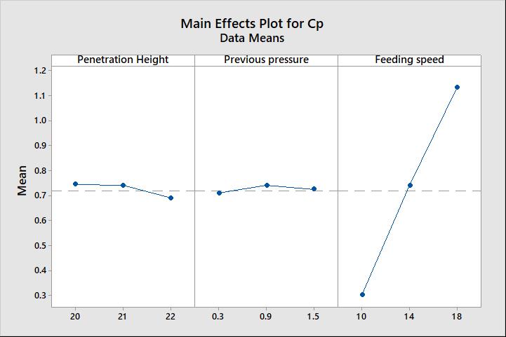
Chart means that values higher than 0.1412 have a significant impact on the CP. In this case, only feeding speed shows a truly impact on the weight variation. In consequence, we can simplify our statistical analysis considering only feeding speed. So, we can get the following, again from Minitab.
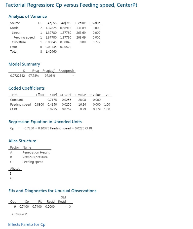
On regression Equation in Uncoded Units, you can see a mathematical model that helps us predicting CP when given a feeding speed. Validity of this model is assured by section Model Summary when you can see an r2 adjusted value of 97.03%. In the field, a value of 80% or more means that model is quite good for predicting.
Now, let’s use the model for defining feeding speed that would allow us to get CP values higher than 1.33. Minitab also helps us to make these predictions.

For feeding speed of 18, CP is 1.13, which, by the way, is the mean of all the 4 values gotten from the DoE runs at 18 speed.

If we want to get CP = 1.34, we need to set speed at 20. If we increase speed, we will get higher CP values, as you can see as follows:
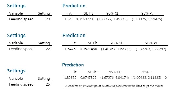
However, we have a constrain: in the field, extrapolating values are not recommended because we do not have certainty if phenomenon behaves at the same way out of the trial boundaries (it is, the range where we were working on).
Certainly, using the model and getting values out of the boundaries, it may give us a clue and just we need to test it. However, a practical constraint would be (and actually is) that maximum speed is not as higher.
So, this will help us to make a decision regarding some options:
1. Simply, increasing feeding speed and looks what happens.
2. Perhaps, it would be needed to set a lower machine speed to increase CP values. In this case, it is just needed to decrease machine speed and evaluating at which one CP is acceptable, taking into account process cost.
3. Reviewing characteristics of the material used to get the slugs: perhaps we have a constrain in the functionality of the materials, and you may need optimize it before keep moving.
In the actual case study, it was observed that material characteristics were the constrain, and the action plan was:
1. Working with current material at lower speed in a temporary way.
2. Rheological characteristics (mainly flow and particle size) were enhanced.
Finally, time required for running DoE and analyzing results was about 4 days: preparing materials, running trials, analyzing data and concluding. Each run lasted by 20 minutes each, in order to get a representative operation time of the machine.
This is a demonstration of the practical usefulness of DoE for saving time and costs. I hope it be useful to you.
